Self-Tracking For Panic: A Deeper Look
In this post, I apply three statistical and machine learning tools to my panic recovery journal data: linear regression/correlation, the Fast Fourier Transform, and maximum entropy modelling.
First, A Word About Tools #
I suppose it is tempting, if the only tool you have is a hammer, to treat everything as if it were a nail.
Now, A Necessary Disclaimer #
My experiment has fewer than 50 samples, which is nowhere near enough to draw statistically significant conclusions. That's not the point. The primary purpose of this post is to demonstrate analysis techniques by example. These same methods can be wielded on larger datasets, where they are much more useful.
Getting Ready #
To follow along with the examples here, you'll need the excellent Python toolkits scipy, matplotlib, and nltk:
$ pip install scipy nltk matplotlibLinear Regression #
What? #
Linear regression answers this question:
What is the line that most closely fits this data?
Given points $ P_i = (x_i, y_i) $, the goal is to find the line $ y = mx + b $ such that some error function is minimized. A common one is the least squares function:
$$
f(m, b) = \sum_{i} \left(y_i - (mx_i + b)\right)^2
$$
The Pearson correlation coefficient $ R $ and p-value $ p $ are also useful here, as they measure correlation and statistical significance.
Why? #
In a self-tracking context, you might ask the following questions:
- Have I been exercising more over time?
- Does exercise affect mood? By how much and in what direction?
Linear regression can help address both questions. However, it can only find linear relationships between datasets. Many dynamic processes are locally linear but not globally linear. For instance, there are practical limits to how much you can exercise in a day, so no linear model with non-zero slope will accurately capture your exercise duration for all time.
The Data #
You can see the code for this analysis here. I look at only the first 31 days, that being the largest consecutive run for which I have data.
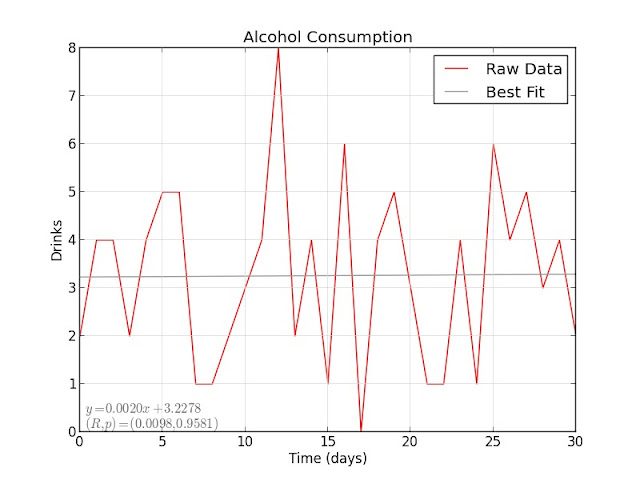
My alcohol consumption did not decrease over time, but rather stayed fairly constant: with $ R = 0.0098 $, there is no correlation between alcohol and time.
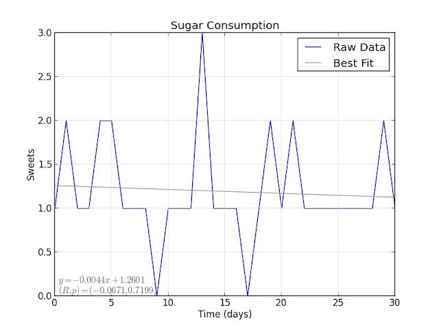
Sugar consumption is a similar story: although the best-fit slope is slightly negative, $ R = -0.0671 $ indicates no correlation over time. It seems that my alcohol and sugar consumption were not modified significantly over the tracking period.
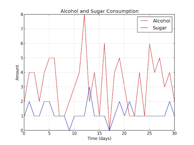
I decided to graph alcohol and sugar together. It looks like they might be related, as the peaks in each seem to coincide on several occasions. Let's test this hypothesis:
The positive slope is more pronounced this time, but $ R = 0.1624 $ still indicates a small degree of correlation. We can also look at the p-value: with $ p = 0.3827 $, it is fairly easy to write this off as a random effect.
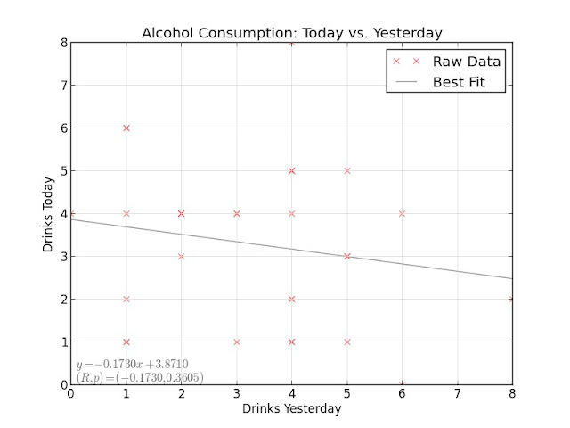
Finally, let's take another look at a question from a previous blog post:
On days where I drink heavily, do I drink less the day after?
There's a negative slope there, but the correlation and p-value statistics are in the same uncertain zone as before. I likely need more data to investigate these last two effects properly.
Fast Fourier Transform #
What? #
Fourier analysis answers this question:
What frequencies comprise this signal?
Given a sequence $ x_n $, a Discrete Fourier Transform (DFT) computes
$$
X_k = \sum_{n=0}^{N-1} x_n \cdot e^{\frac{-2 i \pi k n}{N}}
$$
The $ X_k $ encode the amplitude and phase of frequencies $ \frac{f k}{N} $ Hz, where $ T $ is the time between samples and $ f = 1 / T $ is the sampling frequency.
As described here, the DFT requires $ \mathcal{O}(N^2) $ time to compute. The Fast Fourier Transform (FFT) uses divide-and-conquer on this sum of complex exponentials to compute the DFT in $ \mathcal{O}(N \log N) $ time. Further speedups are possible for real-world signals that are sparse in the frequency domain.
Why? #
In a self-tracking context, you might ask the following questions:
- Do I have regular exercising patterns?
- Do these patterns cycle weekly? bi-weekly? monthly?
- How much does my amount of exercise fluctuate during a cycle?
With the FFT, Fourier analysis can help address these questions. However, it can only find periodic effects. Unlike linear regression, it does not help find trends in your data.
The Data #
You can see the code for this analysis here. Again, I look at the first 31 days to ensure that the frequency analysis is meaningful.
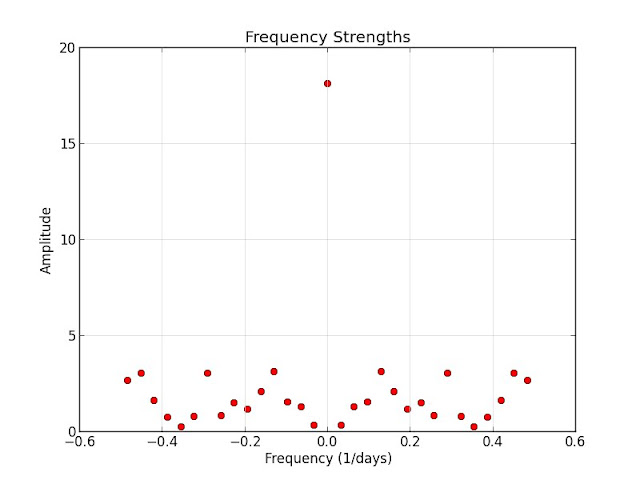
There are some apparent maxima there, but it's hard to tell what they mean. Part of the difficulty is that these are frequencies rather than period lengths, so let's deal with that:
$ python food_fft.py
food_fft.py:32: RuntimeWarning: divide by zero encountered in divide
  for strength, phase, period in sorted(zip(FS, FP, 1.0 / Q))[-5:]:
[2.21 days] 3.0461 (phase=-0.67 days)
[-2.21 days] 3.0461 (phase=-0.67 days)
[7.75 days] 3.1116 (phase=-3.67 days)
[-7.75 days] 3.1116 (phase=-3.67 days)
food_fft.py:33: RuntimeWarning: invalid value encountered in double_scalars
  phase_days = period * (phase / (2.0 * math.pi))
[inf days] 18.1401 (phase=nan days)
If you're not familiar with the Fourier transform, the last line might be a bit mysterious. That corresponds to $ X_0 $, which is just the sum of the original samples:
$$
X_0 = \sum_{n=0}^{N-1} x_n \cdot e^0 = \sum_{n=0}^{N-1} x_n
$$
Other than that, the most pronounced cycles have period lengths of 2.21 days and 7.75 days. The former might be explained by a see-saw drinking pattern, whereas the latter is likely related to the day-of-week effects we saw in the previous post.
Which day of the week? The phase is -3.67 days, and our sample starts on a Monday, placing the first peak on Thursday. The period is slightly longer than a week, though, and the data runs for 31 days, so these peaks gradually shift to cover the weekend.
There are two caveats:
- I have no idea whether a Fourier coefficient of about 3 is significant here. If it isn't, I'm grasping at straws.
- Again, the small amount of data means the frequency domain data is sparse. To accurately test for bi-daily or weekly effects, I need more fine-grained period lengths.
Maximum Entropy Modelling #
What? #
Maximum entropy modelling answers this question:
Given observations of a random process, what is the most likely model for that random process?
Given a discrete probability distribution $ p(X = x_k) = p_k $, the entropy of this distribution is given by
$$
H(p) = \sum - p_k \log p_k
$$
(Yes, I'm conflating the concepts of random variables and probability distributions. If you knew that, you probably don't need this explanation.)
This can be thought of as the number of bits needed to encode outcomes in this distribution. For instance, if I have a double-headed coin, I need no bits: I already know the outcome. Given a fair coin, though, I need one bit: heads or tails?
After repeated sampling, we get observed expected values for $ p_k $; let these be $ p'_k $. Since we would like the model to accurately reflect what we already know, we impose the constraints $ p_k = p'_k $. The maximum entropy model is the model that also maximizes $ H(p') $.
This model encodes what is known while remaining maximally noncommittal on what is unknown.
Adam Berger (CMU) provides a more concrete example. If you're interested in learning more, his tutorial is highly recommended reading.
Why? #
In a self-tracking context, you might ask the following questions:
- Which treatments have the greatest effect in preventing panic attacks? Which have the least effect?
- Today I exercised for at least 30 minutes and had four drinks. Am I likely to get a panic attack?
- What treatments should I try next?
Maximum entropy modelling can help address these questions. It is often used to classify unseen examples, and would be fantastic in a data commons scenario with enough data to provide recommendations to users.
Feature Extraction #
Since I'm now effectively building a classifier, there's an additional step. I need features for my classifier, which I extract from my existing datasets:
train_set = []
dates = set(W).intersection(F)
for ds in dates:
  try:
    ds_data = {
      'relaxation' : bool(int(W[ds]['relaxation'])),
      'exercise' : bool(int(W[ds]['exercise'])),
      'caffeine' : int(F[ds]['caffeine']) > 0,
      'sweets' : int(F[ds]['sweets']) > 1,
      'alcohol' : int(F[ds]['alcohol']) > 4,
      'supplements' : bool(int(F[ds]['supplements']))
    }
  except (ValueError, KeyError):
    continue
  had_panic = P.get(ds) and 'panic' or 'no-panic'
  train_set.append((ds_data, had_panic))
Note that the features listed here are binary. I use my daily goals as thresholds on caffeine, sweets, and alcohol.
(If you know how to get float-valued features working with NLTK, let me know! Otherwise, there's always megam or YASMET.
The Data #
You can see the code for this analysis here. This time I don't care about having consecutive dates, so I use all of the samples.
After building a MaxentClassifier, I print out the most informative features with show_most_informative_features():
  -2.204 exercise==True and label is 'panic'
   1.821 caffeine==True and label is 'panic'
  -0.867 relaxation==True and label is 'panic'
   0.741 alcohol==True and label is 'panic'
  -0.615 caffeine==True and label is 'no-panic'
  -0.537 supplements==True and label is 'panic'
   0.439 sweets==True and label is 'panic'
   0.430 exercise==True and label is 'no-panic'
   0.284 relaxation==True and label is 'no-panic'
   0.233 supplements==True and label is 'no-panic'
Exercise, relaxation breathing, and vitamin supplements help with panic. Caffeine, alcohol, and sweets do not. I knew that already, but this suggests which treatments or dietary factors have greatest impact.
Let's consider the supplements finding more closely. Of the 45 days, I took supplements on all but two. It's dangerous to draw any conclusions from a feature for which there are very few negative samples. This points out some important points about data analysis:
- Know your data: otherwise, you may ascribe undue meaning to outliers or noise.
- Know your features: supplements are probably not a good feature here. A feature inclusion threshold on number of positive and negative samples might be helpful here.
- Beware magic: even when you understand their inner workings, machine learning algorithms can produce results that are difficult to interpret.
Up Next #
In my next post, I look at a panic recovery dataset gathered using qs-counters, a simple utility I built to reduce friction in self-tracking. I perform these same three analyses on the qs-counters dataset, then compare it to the recovery-journal dataset.