Self-Tracking for Panic: Another Dataset
In this post, I perform the same analyses presented in my last post using data from my second panic tracking period. I then test whether my average alcohol and sugar consumption changed measurably between the two tracking periods.
During the second tracking period, I gathered data using qs-counters, a simple utility I built for reducing friction in the recording process.
The Usual Suspects #
Linear Regression #
During the second tracking period, alcohol consumption remained relatively constant:

Sugar consumption is a different story, with a pronounced negative trend:

The evidence to suggest that my alcohol and sugar consumption are linked is also much stronger now:

On the other hand, the previous-day alcohol effect seems to be non-existent:

Fast Fourier Transform #
With more data points, the FFT frequency amplitude plot is more muddled:
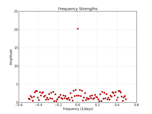
The 2-day and 7-day effects previously "discovered" are nowhere to be found.
Maximum Entropy Modelling #
I didn't record panic attacks during this tracking period. My previous efforts reduced the severity and frequency of these attacks drastically, enough so that the data here would have been extremely sparse.
In the absence of that data, I asked a different question:
What features best predict my exercise patterns?
Here are the top features from MaxentClassifier:
   3.369 caffeine==True and label is 'no-exercise'
  -0.739 sweets==True and label is 'exercise'
   0.399 sweets==True and label is 'no-exercise'
  -0.201 alcohol==True and label is 'exercise'
   0.166 alcohol==True and label is 'no-exercise'
   0.161 relaxation==True and label is 'exercise'
  -0.092 relaxation==True and label is 'no-exercise'
The caffeine finding is misleading. On one of the two days where I entered non-zero caffeine consumption, that was due to a mistake in data entry. (Side note to self: all tools should include an undo feature!) Aside from that, sugar consumption appears to have the strongest negative effect on exercise.
Student's t-test #
What? #
Student's t-test answers this question:
Are these samples significantly different?
More formally, the t-test answers a statistical question about normal distributions: given $ X \sim \mathcal{N}(\mu_X, \sigma_X^2) $ and $ Y \sim \mathcal{N}(\mu_Y, \sigma_Y^2) $, does $ \mu_X = \mu_Y $?
If we let $ Y $ be a known normal distribution centered at rather than taking it from an empirical sample, we also obtain a one-sample t-test for the null hypothesis $ \mu_X = \mu_Y $.
Why? #
In a self-tracking context, you might ask the following questions:
- Did I improve significantly across tracking periods?
- Is my behavior consistent across tracking periods?
Student's t-test can help address both questions.
The Data #
Before using Student's t-test on my alcohol and sugar consumption data from the two tracking periods, I check whether these samples have a roughly normal distribution. The code for normality checking is here.
It helps to visualize the histogram data first:

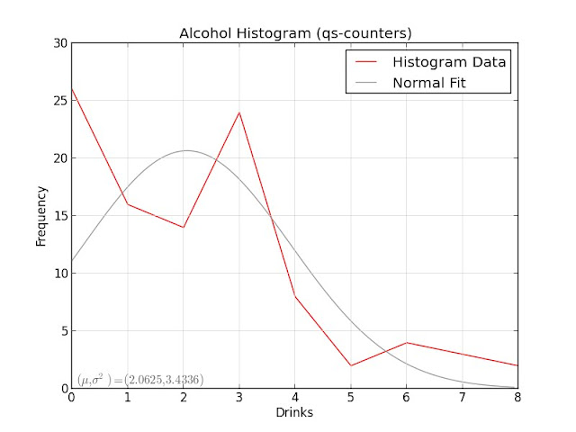

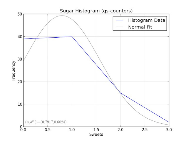
These don't look particularly close to normal distributions, but it's hard to
tell with discrete-valued data. For more evidence, I use the
Shapiro-Wilk statistical normality test:
alcohol, recovery-journal:  (0.944088339805603, 0.10709714889526367)
alcohol, qs-counters:  (0.8849299550056458, 4.6033787270971516e-07)
sugar, recovery-journal:  (0.722859263420105, 2.5730114430189133e-06)
sugar, qs-counters:  (0.8092769384384155, 8.38931979441071e-10)
The null hypothesis for Shapiro-Wilk is that the sample is normally distributed, so these low p-values indicate the opposite: my data isn't normally distributed! Bad news for my attempt to use Student's t-test here.
Nevertheless, I'll barge ahead and run the t-test anyways, just to see what that process looks like with scipy.stats. The code for t-testing is here.
alcohol
==========
avg(A) = 3.26
avg(B) = 2.35
(t, p) = (2.0721, 0.0469)

sweets
==========
avg(A) = 1.19
avg(B) = 1.23
(t, p) = (-0.1969, 0.8453)
If the t-test were useful for this data, it would show that my alcohol consumption was significantly lower during the second tracking period. With such a large drop in average consumption, I'm willing to say that this is a reasonable assertion.
A Question Of Motivation #
By this point, you might be asking:
Why did I even bother with all this analysis when I have so few data points?
Good question! The short answer? It's a learning opportunity. The longer answer is backed by a chain of reasoning:
- As data collection gets easier, the value of data analysis goes up;
- Statistical analysis is hard to impossible for the average user, so they will use whatever tools they can get from app markets and device vendors;
- Most of those tools are built by people who, by trade, are software developers;
- Most developers, even good ones, are typically not that great in the statistics and data analysis department;
- Therefore, as a developer with plans to build self-tracking tools, I owe it to myself and my future users to know this stuff better.
As it turns out, data analysis is hard, period. Picking the right tools is difficult, and picking the wrong ones (like the t-test above!) can easily produce results that appear to be meaningful but are not. In a self-tracking scenario, this problem is often made worse by smaller datasets and uncontrolled conditions.
Thought Experiments #
Repeat Yourself: A Reflection On Self-Tracking And Science #
One criticism often launched at the Quantified Self community is that self-tracking is not scientific enough. For an interesting discussion of the merits and drawbacks of presenting self-experimentation as science, I highly recommend the Open Peer Commentary section of this paper. Some of the broader themes in this debate are also summarized here on the Quantified Self website.
To be fair, there are a host of valid concerns here. For starters, it's very difficult to impose a controlled environment when self-tracking. In a Heisenbergian twist, being mindful of your behavior could modify the behavior you're trying to measure; this effect is discussed briefly by Simon Moore and Joselyn Sellen.
Additionally, a sample population of one is meaningless. Will your approaches work for others? Did you gather the data in a consistent manner? Are your sensors working properly? The usual antidote is to increase the sample population, but then you have another set of problems. Are all participants using the same sensors in the same way? Are they all running the same analyses?
From watching several presentations about self-tracking, there is a curious pattern:
Like any other habit, the tracking habit is hard to maintain.
As a corollary, many tracking experiments consist of multiple tracking periods, these punctuated by relapses of the tracking habit.
Many people interpret these relapses as failures, but they're actually amazing scientific opportunities! These are chances to re-run the same experiment, verifying or confounding results from your earlier tracking periods.
The Predictive Modelling Game #
Predictive modelling could be an interesting component of a habit modification system. Suppose I want to exercise more regularly. First, I select several features that seem likely to influence my exercise patterns, such as:
- Am I travelling? Where am I?
- What foods did I eat? When? How much?
- How positive or negative is my mood?
- Did I schedule time today to exercise?
- Did I exercise yesterday? How much?
Next, I gather some baseline data by tracking these features along with my exercise patterns. I then use that data to train a classifier. Finally, I keep tracking the features, ask the classifier to predict my exercise activity, and play a simple game with myself:
Can I beat the classifier?
That is, can I exercise more often than my existing behavior patterns suggest I should?