The Behavioral Economics of 23AndMe Results
Over the holidays, I received a 23andMe genetic testing kit as a gift. In this post, I'll take a look at my results through the lens of prospect theory, which aims to quantify our perception of risk. 23andMe results estimate your lifetime likelihood of various medical conditions, making them a great dataset for testing out these concepts in behavioral economics.
Prospect Theory: A Quick Example #
Suppose I offer you a bet. I flip a fair coin once. Heads, you gain \$1000; tails, you lose \$900. Do you take the bet? Probability dictates that you should, since you would expect to come out $ (1000 - 900) / 2 = 50 $ dollars ahead.
If you're like most people, though, you have a powerful aversion to losing \$900. This aversion is powerful enough that you'll decline the bet. This only makes sense if losing \$900 has a greater negative value than the positive value of gaining \$1000. In other words, your perception of value is non-linear. This perception underpins many real-world bets that make little sense from an expected utility standpoint:
- Insurance: the buyer takes a small certain loss to avoid the risk of an uncertain and potentially large loss;
- Security: the property owner takes a small certain loss to reduce the risk of an uncertain and potentially large loss;
- Lotteries: the ticket holder takes a small certain loss to try for an extremely unlikely but massive gain.
Prospect theory creates a mathematical framework for understanding our perceptions of value and risk. It's an awesome paper with highly approachable mathematics. Definitely recommended reading for anyone interested in economics, game theory, and the like.
My Disease Risk #
Among other things, 23andMe can estimate your lifetime risk of various diseases. This information is divided into three categories according to whether your risk is highly elevated, highly decreased, or roughly typical:


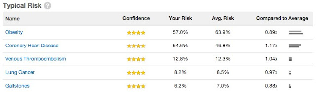
Within each category, the diseases are ordered by decreasing confidence rating, then by decreasing absolute risk. The different confidence levels are as follows:
- Preliminary Research: fewer than 100 people studied
- Preliminary Research: fewer than 750 people studied
- Preliminary Research: a single study with 750+ participants
- Established Research: multiple studies with 750+ participants
The 23andMe dashboard doesn't show estimated risk for lower-confidence findings, but I can fetch that information through their API.
Armed with my raw risk data, I can now play around with a pair of alternative disease rankings. As an anchoring point, here's my disease ranking by absolute risk:
$ python risksort.py risk < risks.json
 1                                            Obesity 0.5701
 2                             Coronary Heart Disease 0.5464
 3                                Atrial Fibrillation 0.3392
 4                                    Prostate Cancer 0.2602
 5                   Age-related Macular Degeneration 0.2459
 6                                    Type 2 Diabetes 0.1969
 7                             Venous Thromboembolism 0.1279
 8                                        Lung Cancer 0.0823
 9                                          Psoriasis 0.0708
10                                         Gallstones 0.0618
11                                Alzheimer's Disease 0.0493
12                                  Colorectal Cancer 0.0417
13                             Chronic Kidney Disease 0.0356
14                               Rheumatoid Arthritis 0.0300
15                             Restless Legs Syndrome 0.0245
16                               Exfoliation Glaucoma 0.0217
17                                           Melanoma 0.0216
18                                    Type 1 Diabetes 0.0137
19                                Parkinson's Disease 0.0109
20                                 Ulcerative Colitis 0.0066
21                                 Multiple Sclerosis 0.0047
22          Esophageal Squamous Cell Carcinoma (ESCC) 0.0043
23     Stomach Cancer (Gastric Cardia Adenocarcinoma) 0.0028
24                                    Crohn's Disease 0.0016
25                                   Bipolar Disorder 0.0015
26                                     Celiac Disease 0.0005
27               Scleroderma (Limited Cutaneous Type) 0.0005
28                          Primary Biliary Cirrhosis 0.0004
29                                      Breast Cancer 0.0000
30               Lupus (Systemic Lupus Erythematosus) 0.0000
The alternative ranking metric code can be found here.
Relative-Risk Sorting #
An obvious ranking metric is relative risk, which is already provided in the disease listing.
$ python risksort.py relative_risk < risks.json
 1                   Age-related Macular Degeneration 3.7542
 2                               Exfoliation Glaucoma 2.8933
 3                                   Bipolar Disorder 1.5000
 4                                    Prostate Cancer 1.4593
 5                                 Multiple Sclerosis 1.3824
 6                                    Type 1 Diabetes 1.3431
 7                               Rheumatoid Arthritis 1.2605
 8                             Restless Legs Syndrome 1.2500
 9                                Atrial Fibrillation 1.2494
10     Stomach Cancer (Gastric Cardia Adenocarcinoma) 1.2174
11          Esophageal Squamous Cell Carcinoma (ESCC) 1.1944
12                             Coronary Heart Disease 1.1665
13                             Venous Thromboembolism 1.0365
14                             Chronic Kidney Disease 1.0349
15                                        Lung Cancer 0.9728
16                                            Obesity 0.8926
17                                         Gallstones 0.8766
18                                 Ulcerative Colitis 0.8571
19                                    Type 2 Diabetes 0.7656
20                                           Melanoma 0.7552
21                                  Colorectal Cancer 0.7500
22               Scleroderma (Limited Cutaneous Type) 0.7143
23                                Alzheimer's Disease 0.6885
24                                Parkinson's Disease 0.6770
25                                          Psoriasis 0.6238
26                          Primary Biliary Cirrhosis 0.5000
27                                     Celiac Disease 0.4167
28                                    Crohn's Disease 0.3019
29                                      Breast Cancer 0.0000
30               Lupus (Systemic Lupus Erythematosus) 0.0000
Perceived Relative-Risk Sorting #
In prospect theory, a probability $ p $ has perceived weight $ w(p) $. In Advances in Prospect Theory: Cumulative Representation of Uncertainty, Tversky and Kahneman fit $ w $ to observed results for subjects evaluating bets similar to the one listed above:


The corresponding equations are
$$
w^+(p) = \frac{p^{0.61}}{(p^{0.61} + (1-p)^{0.61})^{\frac{1}{0.61}}}
$$
for positive prospects and
$$
w^-(p) = \frac{p^{0.69}}{(p^{0.69} + (1-p)^{0.69})^{\frac{1}{0.69}}}
$$
for negative prospects. If my risk is $ p_0 $ and the general risk is $ p $, I can define my perceived relative risk as
$$
r = \frac{w^+(p_0)}{w^+(p)}
$$
if $ p_0 < p $ (I consider decreased risk as a positive prospect!) and
$$
r = \frac{w^-(p_0)}{w^-(p)}
$$
otherwise. The resulting rankings are pretty close to ordinary relative risk, but not identical:
$ diff <(python risksort.py relative_risk < risks.json \
  | cut -c-53) <(python risksort.py perceived_relative_risk < risks.json | cut -c-53)
13,14c13,14
< 13                             Venous Thromboembolism
< 14                             Chronic Kidney Disease
---
> 13                             Chronic Kidney Disease
> 14                             Venous Thromboembolism
16,17c16,17
< 16                                            Obesity
< 17                                         Gallstones
---
> 16                                         Gallstones
> 17                                            Obesity
20,23c20,23
< 20                                           Melanoma
< 21                                  Colorectal Cancer
< 22               Scleroderma (Limited Cutaneous Type)
< 23                                Alzheimer's Disease
---
> 20                                  Colorectal Cancer
> 21                                           Melanoma
> 22                                Alzheimer's Disease
> 23               Scleroderma (Limited Cutaneous Type)
The difference is due to distortion of small probabilities.
Further Ideas #
So far, I've only used the probability weighting functions from prospect theory. I could also assign values to each disease:
- Financial: how much does this disease cost to treat on average?
- Reduced Life Expectancy: how many years of potential life do these diseases claim on average?
- Lifestyle: how much impact would this have on my highly active lifestyle? On others who might have to support me?
This is definitely morbid, but it's also potentially worthwhile. After all, insurance companies make very detailed estimates of our risk. They will certainly incorporate genetic data into their models as soon as it's legal to do so. If we want to make more informed decisions in situations involving risk, from medical insurance to lottery tickets, it helps to understand how we value different outcomes.
Appendix: How To Use The 23andMe API #
The 23andMe API is actually quite easy to use, and their documentation is excellent. Nevertheless, I'll list the flow I went through to get my genetic disease risk data. If you're unfamiliar with OAuth 2.0, the Google API docs include this primer complete with cute stick figure diagrams.
First, I log into the API console and create an app. This gives me the client_id and client_secret parameters I need to initiate the flow. Looking at the 23andMe API reference, I see that I need permissions under the analyses scope, so I request that by visiting
https://api.23andme.com/authorize/?redirect_uri=http://localhost:5000/receive_code/&response_type=code&client_id=<client_id>&scope=analysesin the browser. I'm redirected to
http://localhost:5000/receive_code/?code=<code>which gives me the auth code I need to request a token:
$ curl https://api.23andme.com/token/ \
  -d client_id=<client_id> \
  -d client_secret=<client_secret> \
  -d code=<code> \
  -d grant_type=authorization_code \
  -d "redirect_uri=http://localhost:5000/receive_code/" \
  -d scope=analyses > token.json
$ jsonpp token.json
{
  "access_token": "<access_token>"
  "token_type": "bearer",
  "expires_in": 86400,
  "refresh_token": "<refresh_token>"
  "scope": "analyses"
}
Finally, I use my shiny new access_token to get my genetic risk data:
$ curl https://api.23andme.com/1/risks/ \
  -H "Authorization: Bearer <access_token>" > risks.json
$ jsonpp risks.json | head
[
  {
    "id": "6d2de403675a0d07",
    "risks": [
      {
        "description": "Atrial Fibrillation",
        "risk": 0.3392,
        "population_risk": 0.2715,
        "report_id": "atrialfib"
      },